
Formatting in exel
Formatting in excel is used to present data in more presentable form so that it is easily readable.
NOTE: In excel, by default numbers are right aligned and string values are left aligned.
TABLE 1
|
EmpID |
Names |
Date |
Salary |
|
0001 |
Robert |
43101 |
340098 |
|
0002 |
John |
43102 |
34562 |
|
0003 |
Philips |
43103 |
76543 |
|
0004 |
Andrew |
43104 |
85214 |
|
0005 |
Rose |
43105 |
52413 |
|
0006 |
Jill |
43106 |
78541 |
|
0007 |
Johns |
43107 |
539561 |
|
0008 |
Jordan |
43108 |
548000 |
|
0009 |
Smith |
43109 |
92000 |
|
0010 |
Ahil |
43110 |
3621000 |
- USING PREDEFINED FORMATS
- Formatting Date-
STEP 1-Select the column you want to format. In this case it is Date
STEP 2-Go to Home Tab->Number
Here you will see two formats i.e. Short date and Long date,
You can select any format. I have selected Long Format.
|
EmpID |
Names |
Date |
Salary |
|
0001 |
Robert |
Monday, 1 January 2018 |
340098 |
|
0002 |
John |
Tuesday, 2 January 2018 |
34562 |
|
0003 |
Philips |
Wednesday, 3 Januar 2018 |
76543 |
|
0004 |
Andrew |
Thursday, 4 January 2018 |
85214 |
|
0005 |
Rose |
Friday, 5 January 2018 |
52413 |
|
0006 |
Jill |
Saturday, 6 January 2018 |
78541 |
|
0007 |
Johns |
Sunday, 7 January 2018 |
539561 |
|
0008 |
Jordan |
Monday, 8 January 2018 |
548000 |
|
0009 |
Smith |
Tuesday, 9 January 2018 |
92000 |
|
0010 |
Ahil |
Wednesday,10January2018 |
3621000 |
- Formatting Salary
Step 1 is same as above.
Step 2- Number->Select Currency. You can use “,” separator to make is more readable from the option displayed on NUMBER tab.
|
EmpID |
Names |
Date |
Salary |
|
0001 |
Robert |
Monday, 1 January 2018 |
$340,098.00 |
|
0002 |
John |
Tuesday, 2 January 2018 |
$34,562.00 |
|
0003 |
Philips |
Wednesday, 3 Januar2018 |
$76,543.00 |
|
0004 |
Andrew |
Thursday, 4 January 2018 |
$85,214.00 |
|
0005 |
Rose |
Friday, 5 January 2018 |
$52,413.00 |
|
S0006 |
Jill |
Saturday, 6 January 2018 |
$78,541.00 |
|
0007 |
Johns |
Sunday, 7 January 2018 |
$539,561.00 |
|
0008 |
Jordan |
Monday, 8 January 2018 |
$548,000.00 |
|
0009 |
Smith |
Tuesday, 9 January 2018 |
$92,000.00 |
|
0010 |
Ahil |
Wednesday,10 January2018 |
$3,621,000.00 |
|
|
|
|
|
There are many predefined formats given in “Number Format”. You can try each of them.
- CUSTOM FORMATTING
DATE
We can use custom formatting to customize the data according to our needs.
Let us consider the same Table i.e. Table 1
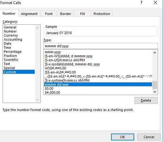
For Ex. We want to show the date in (“January 01’2018”)
STEP 1- Home->Number->More Number Formats->Custom
STEP 2- In the Type section, you can write your own format
Some Rules:
For month
If you write
mm – 01 (You will get the month number)
mmm – Jan (You will get the abbreviated month)
mmmm – January (Full month)
For Date
dd – 01 (you will get the date)
ddd – Mon (You will get the abbreviated day)
dddd – Monday (Full day)
For YEAR
y – 18 (year will be displayed)
yyy – 2018 (complete year will be displayed)
Using the above rules – “mmmm dd’yyy”
STEP 3 - After clicking OK
OUTPUT
|
EmpID |
Names |
Date |
Salary |
|
0001 |
Robert |
January 01'2018 |
$340,098.00 |
|
0002 |
John |
January 02'2018 |
$34,562.00 |
|
0003 |
Philips |
January 03'2018 |
$76,543.00 |
|
0004 |
Andrew |
January 04'2018 |
$85,214.00 |
|
0005 |
Rose |
January 05'2018 |
$52,413.00 |
|
0006 |
Jill |
January 06'2018 |
$78,541.00 |
|
0007 |
Johns |
January 07'2018 |
$539,561.00 |
|
0008 |
Jordan |
January 08'2018 |
$548,000.00 |
|
0009 |
Smith |
January 09'2018 |
$92,000.00 |
|
0010 |
Ahil |
January 10'2018 |
$3,621,000.00 |
CURRENCY
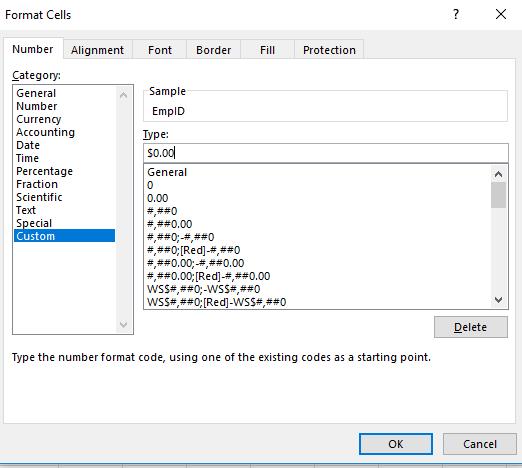
STEP 1- Home->Number->More Number Formats->Custom
STEP 2- In the Type section, you can write your own format
STEP 3- Example Format “$0.00”
Some Rules:
“0” – Zero represents the number itself
“.” – Dot will specify decimal point & number of zeroes after decimal represent, number of places we want after the decimal.
For number format we can use “0” – it will represent the number itself & all type of formatting can be done in it as we have done in currency
OUTPUT
|
EmpID |
Names |
Date |
Salary |
|
0001 |
Robert |
January 01'2018 |
$340098.00 |
|
0002 |
John |
January 02'2018 |
$34562.00 |
|
0003 |
Philips |
January 03'2018 |
$76543.00 |
|
0004 |
Andrew |
January 04'2018 |
$85214.00 |
|
0005 |
Rose |
January 05'2018 |
$52413.00 |
|
0006 |
Jill |
January 06'2018 |
$78541.00 |
|
0007 |
Johns |
January 07'2018 |
$539561.00 |
|
0008 |
Jordan |
January 08'2018 |
$548000.00 |
|
0009 |
Smith |
January 09'2018 |
$92000.00 |
|
0010 |
Ahil |
January 10'2018 |
$3621000.00 |
NUMBER
For number format we can use “0” – it will represent the number itself & all type of formatting can be done in it as we have done in currency.
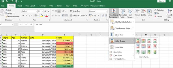
- CONDITIONAL FORMATTING
Conditional formatting is used for highlighting important stuff in the data. Excel provide us with default conditional formats as well as custom options
PREDEFINED FORMATS
STEP 1 – Home->Styles->Conditional Formatting. In this tab, we have several options. Let’s have a look on some of them.
TABLE 2
|
EmpID |
Age |
Names |
Date |
Salary |
|
0001 |
40 |
Robert |
January 01'2018 |
$340098.00 |
|
0002 |
36 |
John |
January 02'2018 |
$34562.00 |
|
0003 |
35 |
Philips |
January 03'2018 |
$76543.00 |
|
0004 |
25 |
Andrew |
January 04'2018 |
$85214.00 |
|
0005 |
27 |
Rose |
January 05'2018 |
$52413.00 |
|
0006 |
30 |
Jill |
January 06'2018 |
$78541.00 |
|
0007 |
45 |
Johns |
January 07'2018 |
$539561.00 |
|
0008 |
30 |
Jordan |
January 08'2018 |
$548000.00 |
|
0009 |
22 |
Smith |
January 09'2018 |
$92000.00 |
|
0010 |
29 |
Ahil |
January 10'2018 |
$3621000.00 |
1.Highlight cell rules
In this tab we have options like Greater than, Less than, between etcetera.
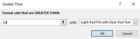
Q1. Suppose we want to highlight that cell which has age greater than 29
STEP 1- Select Age column
STEP 1 - Home->Styles->Conditional Formatting->Greater Than
STEP 2 – Enter the desired value
STEP 3 – Press OK
OUTPUT
|
EmpID |
Age |
Names |
Date |
Salary |
|
0001 |
40 |
Robert |
January 01'2018 |
$340098.00 |
|
0002 |
36 |
John |
January 02'2018 |
$34562.00 |
|
0003 |
35 |
Philips |
January 03'2018 |
$76543.00 |
|
0004 |
25 |
Andrew |
January 04'2018 |
$85214.00 |
|
0005 |
27 |
Rose |
January 05'2018 |
$52413.00 |
|
0006 |
30 |
Jill |
January 06'2018 |
$78541.00 |
|
0007 |
45 |
Johns |
January 07'2018 |
$539561.00 |
|
0008 |
30 |
Jordan |
January 08'2018 |
$548000.00 |
|
0009 |
22 |
Smith |
January 09'2018 |
$92000.00 |
|
0010 |
29 |
Ahil |
January 10'2018 |
$3621000.00 |
TOP/BOTTOM RULES
Q2. Suppose we want to highlight top 2 values in Salary column
- By default, it will highlight 10 values.
STEP 1 – Select the column you want to apply formatting on, in this case (Salary)
STEP 2 - Home->Styles->Conditional Formatting->Top 10 items
STEP 3 – Enter the desired value
STEP 4 – Press OK
|
EmpID |
Age |
Names |
Date |
Salary |
|
0001 |
40 |
Robert |
January 01'2018 |
$340098.00 |
|
0002 |
36 |
John |
January 02'2018 |
$34562.00 |
|
0003 |
35 |
Philips |
January 03'2018 |
$76543.00 |
|
0004 |
25 |
Andrew |
January 04'2018 |
$85214.00 |
|
0005 |
27 |
Rose |
January 05'2018 |
$52413.00 |
|
0006 |
30 |
Jill |
January 06'2018 |
$78541.00 |
|
0007 |
45 |
Johns |
January 07'2018 |
$539561.00 |
|
0008 |
30 |
Jordan |
January 08'2018 |
$548000.00 |
|
0009 |
22 |
Smith |
January 09'2018 |
$92000.00 |
|
0010 |
29 |
Ahil |
January 10'2018 |
$3621000.00 |
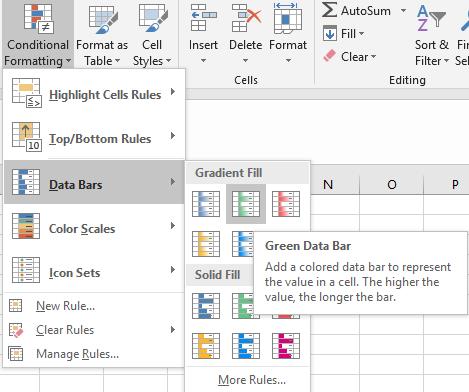
DATA BARS
It is used to show the data in bars, to make it more appealing
Q3. Suppose we want to show Salary in the form of bars.
STEP 1 – Select the column you want to apply formatting on, in this case (Salary)
STEP 2 - Home->Styles->Conditional Formatting->Data bars
STEP 3 – Enter the desired value
STEP 4 – Press OK
OUTPUT
It takes the largest value as a reference to display other values
COLOR SCALES
3-Color scales calculate the 50th percentile i.e. the cell with the minimum value is colored red, the cell that contains middle value is colored yellow and the cell with the maximum value is colored green.
ICON SETS
It can be applied in the same way as color scales.