PIVOT TABLES
A pivot table is used to summarize the data. Whenever we want to show the data in summarized form, when we don’t want to view the complete data, we use pivot tables.
It can automatically show sum, count, average, total and can be used for all type of sorting.
How to make a pivot table?
Step 1: Select the data
Step 2: Go to insert Tab and select the option Pivot table.
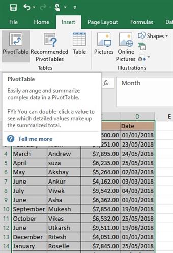
Step 3: A window will pop up that contains the following options.
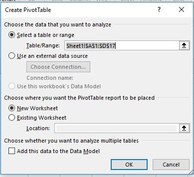
First field is the range, the range we have selected to build pivot table on.
The second option is where you want to create the pivot table either in the same worksheet or new worksheet. One can select ant of them.
Once all this is done, a new sheet will open that will contain an empty pivot table incase you have selected the New Worksheet option.
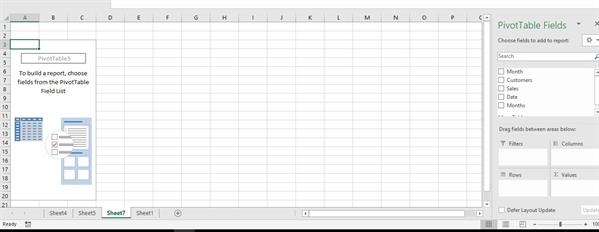
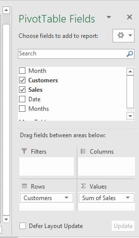
On the right side you will see a Pivot Table Fields. Under the search option you will see that all the headers of the selected data are coming. All you need to do is Drag and Drop
We are provided with four tabs:
Filters: Place that field in this area in which you want to insert filters.
Columns: Place that field in this area that you want to show column wise.
Rows: Place that field in this area that you want to show in rows.
Values: Place that field in this area in which you want to do some sought of calculations.
Let us understand this with an example
Suppose we have this table.
|
Month |
Customers |
Sales |
Date |
|
January |
Anjali |
$6,500.00 |
01/01/2018 |
|
February |
Ridhi |
$4,251.00 |
23/05/2018 |
|
March |
Andrew |
$7,895.00 |
24/05/2018 |
|
April |
suza |
$6,235.00 |
25/05/2018 |
|
May |
Akshay |
$5,264.00 |
02/03/2018 |
|
June |
Ankur |
$4,162.00 |
03/03/2018 |
|
July |
Vivek |
$9,542.00 |
04/03/2018 |
|
June |
Asha |
$6,362.00 |
01/01/2018 |
|
September |
Mukesh |
$7,854.00 |
19/08/2018 |
|
October |
Vikas |
$6,532.00 |
25/05/2018 |
|
June |
Utkarsh |
$9,511.00 |
19/08/2018 |
|
December |
Ritesh |
$4,051.00 |
01/01/2018 |
|
January |
Roselle |
$7,845.00 |
25/05/2018 |
|
February |
Kelly |
$2,546.00 |
18/12/2018 |
|
May |
Maria |
$5,682.00 |
19/12/2018 |
|
January |
Rohit |
$7,500.00 |
20/12/2018 |
In this example I have dragged Customers field in Rows and Sales in Values. By default, Pivot tables calculate the sum of fields that are dragged into values.
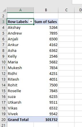
So, we can see customer names in rows and by default it is showing the grand totals.
Another variation could be:
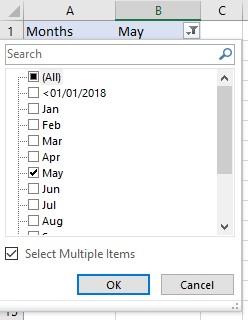
You can drag Month into Filters i.e. it will not show all the months together.
Rather it will show us a filter and we can filter months from it i.e. we can show only that months that we desire for.
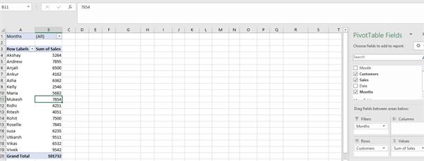
Right now, it is showing all months, we can filter accordingly.
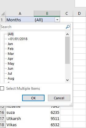
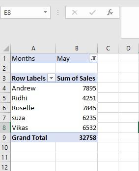
For example, I want to show results for month May. I can select “ Select Multiple Items” and then we choose month May by checking it.
Results
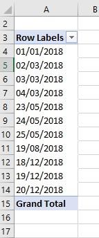
- We can group and ungroup fields
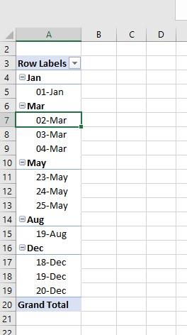
For example, if I want to group dates. Excel provides us with several options, Dates can be grouped into months, years, quarters etcetera. Firstly, drag Date into rows.
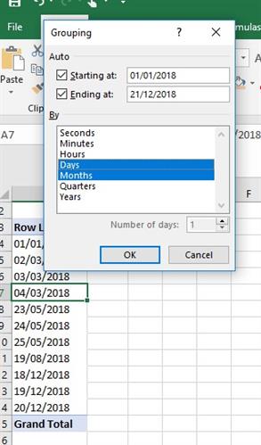
In order to group, right click on the table and choose the option of “Group”
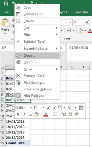
A pop up will appear as shown below. Then we can choose the desired value that we want to show. One can choose multiple options. If we choose Days and Months, then click Ok.
Output
Now it is showing, months with date.